Understanding Time Decay in Commodity Options

Time decay, commonly referred to as theta in options trading, is a central factor in determining the value of commodity options over their lifespan. Commodity options derive their value from underlying physical or futures markets such as crude oil, gold, natural gas, agricultural products, and industrial metals. Like all options, they are classified as wasting assets, meaning that their value declines as time elapses, assuming all other variables remain constant. This gradual reduction in value has significant implications for both short-term and long-term option holders.

An understanding of time decay is necessary not only for directional traders but also for hedgers, institutional participants, and portfolio managers who use commodity options to manage price exposure. While volatility, underlying price movements, and interest rates influence options pricing, time decay operates continuously and predictably. Its impact differs materially between short-dated and long-dated options, shaping strategy selection and risk management decisions.

What Is Time Decay?

Time decay reflects the portion of an option’s price attributable to the time remaining until expiration. An option’s premium consists of two primary components: intrinsic value and extrinsic value. Intrinsic value represents the amount by which an option is in-the-money. Extrinsic value, often called time value, accounts for the probability that the option may gain intrinsic value before expiration.

Theta measures the rate at which this extrinsic value declines with the passage of time. If an option has a theta of -0.05, it will theoretically lose $0.05 per day, all else being equal. Importantly, time decay is non-linear. The erosion of value accelerates as the option approaches expiration because the remaining opportunity for favorable price movement diminishes more rapidly during the final weeks of its life.

Commodity options often exhibit distinctive time decay characteristics because their underlying markets can experience abrupt changes driven by weather patterns, geopolitical events, production shifts, and macroeconomic policies. Nevertheless, regardless of the underlying cause of price movement, time inexorably reduces extrinsic value.

The Structure of Commodity Options Pricing

To understand the practical significance of time decay, it is useful to examine how commodity options are structured. Most commodity options are written on futures contracts rather than directly on physical commodities. This structure introduces additional considerations such as futures expiration cycles, storage costs, seasonal patterns, and forward curves.

Commodity markets frequently display either contango or backwardation, depending on supply-demand dynamics. While these conditions primarily affect futures pricing, they also influence option premiums by shaping expectations of future price movements. Time decay interacts with these market structures by continuously reducing the premium attached to future uncertainty.

For example, options on agricultural commodities often experience heightened implied volatility ahead of planting or harvest seasons. As these key periods pass, uncertainty may decline, which, combined with accelerating time decay, can quickly deflate option premiums.

Mathematics of Time Decay

Theta is one of several “Greeks” used to measure option sensitivity. In formal option pricing models such as Black-Scholes or Black-76 (frequently used for commodity futures options), theta is derived as the partial derivative of the option price with respect to time.

The non-linear nature of time decay is central. During the early life of a long-term option, daily erosion is relatively modest because substantial time remains for favorable movement. As expiration approaches, each day represents a larger proportion of the remaining lifespan. Consequently, the rate of decay increases sharply during the final month and even more so during the last week.

Graphically, time decay follows a curve rather than a straight line. The curve is relatively flat in the early stages and steepens significantly near expiration. This effect is particularly pronounced for at-the-money options, which consist almost entirely of extrinsic value.

Impact on Short-Term Commodity Options

Short-term commodity options typically have expirations ranging from a few weeks to three months. Because their duration is limited, a significant portion of their premium reflects near-term expectations of volatility. As time passes, the ability of the underlying commodity price to make meaningful moves diminishes quickly.

The accelerated time decay of short-term options has several practical consequences. First, at-the-money options lose value rapidly when the underlying commodity remains stable. For instance, a crude oil option with 20 days to expiration may experience a substantial decline in premium over the course of a week if prices fail to move.

Second, short-term options are highly sensitive to immediate price fluctuations. Small changes in the underlying commodity can temporarily offset time decay. However, if the expected move does not materialize quickly, the effect of theta may outweigh gains from price movement.

Third, short-term option buyers face a narrow opportunity window. Even accurate directional forecasts must materialize promptly to overcome accelerating theta. As expiration nears, the option’s extrinsic value compresses sharply, leaving little room for recovery if the trade moves temporarily against the holder.

Commodity markets such as natural gas and agricultural products often experience sudden price spikes triggered by unexpected weather forecasts or supply disruptions. Short-term options can capture such moves efficiently, but the decay profile demands precise timing.

Impact on Long-Term Commodity Options

Long-term commodity options, sometimes extending beyond one year, behave differently due to their extended time horizon. In these instruments, time decay progresses at a slower daily rate during the early and middle portions of their lifespan.

Because substantial time remains for the commodity price to move, extrinsic value erodes gradually. This characteristic provides traders and hedgers with greater flexibility in managing their positions. A temporary adverse price movement does not necessarily render the position unrecoverable, as sufficient time remains for adjustment or improvement.

Long-term options are commonly used by producers, consumers, and institutional investors who wish to establish strategic hedges. For example, a mining company might purchase long-dated put options on copper to protect against prolonged price declines, while retaining upside exposure.

Although daily theta is smaller for long-term options, the total dollar amount of time decay over the life of the contract is substantial. Since the premium paid for long-dated options is typically higher, the cumulative erosion can represent a significant cost if the option remains out-of-the-money.

Comparative Analysis of Short-Term and Long-Term Decay

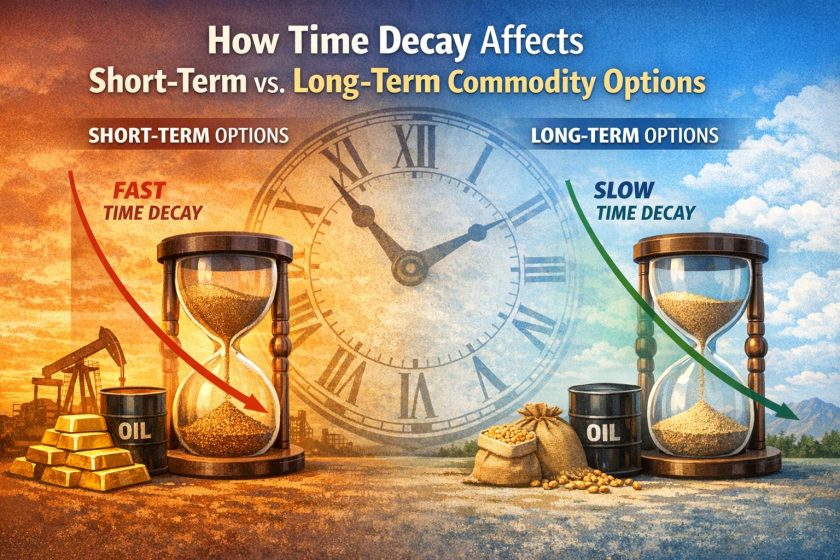
The key distinction between short- and long-term options lies in the distribution of time value across the contract’s life. Short-term options concentrate time decay into a compressed timeframe, leading to noticeable daily losses as expiration nears. Long-term options distribute the decay more evenly across months or years.

In practical terms, consider an at-the-money gold option with two weeks to expiration and another with twelve months remaining. The short-dated option may lose several percentage points of its value each day in the absence of price movement. The long-dated option, in contrast, might experience a comparatively modest daily reduction.

However, the long-term option’s premium is much larger. Therefore, while percentage decay is slower, the absolute dollar decline can still be meaningful over extended periods. The choice between short and long durations depends on capital allocation preferences, risk tolerance, and expectations regarding timing.

Another distinction arises in volatility sensitivity. Longer-term options often have greater vega exposure, meaning changes in implied volatility can offset or amplify the effects of time decay. Short-term options, while also influenced by volatility, are dominated more heavily by theta during the final weeks.

Interaction with Volatility

Time decay does not operate in isolation. Implied volatility plays a central role in determining how quickly an option’s time value may erode. When implied volatility rises, option premiums expand, potentially offsetting the daily impact of theta. Conversely, declining volatility accelerates premium reduction.

Commodity markets frequently exhibit volatility cycles. For example, crude oil may display elevated implied volatility during geopolitical tension, which later contracts as uncertainty subsides. A short-term option purchased during heightened volatility may experience losses from both declining volatility and time decay, even if the underlying price stabilizes.

Long-term options are also affected by volatility shifts, but their slower time decay may provide greater opportunity for volatility recovery. In both cases, traders must assess not only expected price direction but also the volatility environment.

The Role of Moneyness

The degree to which an option is in-the-money, at-the-money, or out-of-the-money significantly influences time decay. At-the-money options possess the greatest extrinsic value and therefore experience the most pronounced time decay. Deep in-the-money options contain higher intrinsic value, reducing the proportion of time value subject to erosion.

Out-of-the-money options, common in speculative commodity trading, may lose value rapidly if the underlying fails to move toward the strike price. In short-term contracts, this erosion can be swift and decisive.

For long-term contracts, out-of-the-money options retain meaningful time value over extended periods, but their sensitivity to directional movement remains substantial. The interaction between moneyness and duration adds complexity to position analysis.

Strategic Considerations

Successful commodity options trading requires integrating time decay into broader strategy design. Buyers of options must anticipate sufficient price movement within a defined timeframe to offset the predictable loss of extrinsic value. Sellers of options, by contrast, may intentionally seek to benefit from theta by collecting premium and allowing time to erode the contract’s value.

Short-term strategies often aim to exploit anticipated volatility around specific events such as government inventory reports, central bank decisions, or seasonal weather updates. These strategies require careful timing because the rapid onset of time decay can quickly reduce profitability if expectations are delayed.

Long-term strategies may focus on structural supply-demand trends in commodities. Investors expecting sustained growth in electric vehicle production, for example, may use long-dated options to gain exposure to lithium or copper price movements. The slower decay profile provides flexibility but requires patience.

In hedging applications, producers and consumers weigh the cost of time decay against the benefit of price certainty. Long-dated protective options provide extended security but may require significant premium expenditure. Decision-makers must evaluate whether the insurance value justifies the time-based cost.

Risk Management Implications

Time decay introduces predictable risk that must be accounted for in portfolio management. Monitoring theta exposure enables traders to understand how much value a position is expected to lose daily. When holding multiple positions across different maturities, aggregate theta may significantly influence overall performance.

Short-term options demand close monitoring because of their accelerating decay. Positions approaching expiration often require adjustment, closure, or exercise decisions. Long-term options, while less sensitive on a daily basis, should still be reviewed regularly to ensure the initial thesis remains valid.

Risk management also involves recognizing that time decay cannot be eliminated through diversification. Every long option position experiences theta. Balancing long and short option positions may offset some exposure, but directional and volatility risks remain.

Practical Examples in Commodity Markets

Consider a natural gas trader anticipating increased demand due to seasonal temperature forecasts. Purchasing a short-term call option may offer leveraged exposure. If the anticipated demand surge occurs promptly, gains may exceed time decay losses. If weather patterns shift unexpectedly, the option’s value may erode rapidly as expiration approaches.

In contrast, an agricultural producer concerned about multi-year price weakness might purchase long-dated put options. Although daily time decay is limited initially, the producer incurs a gradual cost for maintaining protection. If unfavorable conditions persist, the option may gain intrinsic value, offsetting the premium expense.

These examples illustrate how time decay interacts with real-world commodity dynamics. The appropriate duration depends on the alignment between price expectations and the anticipated timeline for change.

Conclusion

Time decay is a fundamental element of commodity options pricing, shaping outcomes for both short-term and long-term positions. As a measure of the steady erosion of extrinsic value, theta operates continuously and accelerates as expiration approaches. Short-term options experience concentrated and rapid decay, requiring timely price movement to remain profitable. Long-term options distribute decay more gradually, offering strategic flexibility but involving higher upfront premiums.

An informed approach to commodity options trading requires integrating time decay analysis with considerations of volatility, moneyness, market structure, and risk tolerance. By understanding how different maturities respond to the passage of time, market participants can more effectively align their strategies with their objectives in dynamic commodity markets.

This article was last updated on: April 25, 2026